Gradient descent
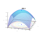
[1] Gradient descent should not be confused with local search algorithms, although both are iterative methods for optimization.[3][4] Its convergence properties for non-linear optimization problems were first studied by Haskell Curry in 1944,[5] with the method becoming increasingly well-studied and used in the following decades.It is possible to guarantee the convergence to a local minimum under certain assumptions on the functionWe see that gradient descent leads us to the bottom of the bowl, that is, to the point where the value of the functionTherefore, the path down the mountain is not visible, so they must use local information to find the minimum.If they were trying to find the top of the mountain (i.e., the maximum), then they would proceed in the direction of steepest ascent (i.e., uphill).However, assume also that the steepness of the hill is not immediately obvious with simple observation, but rather it requires a sophisticated instrument to measure, which the persons happen to have at the moment.The difficulty then is choosing the frequency at which they should measure the steepness of the hill so not to go off track.The amount of time they travel before taking another measurement is the step size.Philip Wolfe also advocated using "clever choices of the [descent] direction" in practice.The first term in square brackets measures the angle between the descent direction and the negative gradient.Gradient descent can be used to solve a system of linear equations reformulated as a quadratic minimization problem.the Euclidean norm is used, in which case The line search minimization, finding the locally optimal step sizeon every iteration, can be performed analytically for quadratic functions, and explicit formulas for the locally optimal), while the convergence of conjugate gradient method is typically determined by a square root of the condition number, i.e., is much faster.Both methods can benefit from preconditioning, where gradient descent may require less assumptions on the preconditioner.[7] That gradient descent works in any number of dimensions (finite number at least) can be seen as a consequence of the Cauchy-Schwarz inequality, i.e. the magnitude of the inner (dot) product of two vectors of any dimension is maximized when they are colinear.The gradient descent can take many iterations to compute a local minimum with a required accuracy, if the curvature in different directions is very different for the given function.The main examples of such optimizers are Adam, DiffGrad, Yogi, AdaBelief, etc.An example is the BFGS method which consists in calculating on every step a matrix by which the gradient vector is multiplied to go into a "better" direction, combined with a more sophisticated line search algorithm, to find the "best" value ofFor extremely large problems, where the computer-memory issues dominate, a limited-memory method such as L-BFGS should be used instead of BFGS or the steepest descent.Gradient descent can be viewed as applying Euler's method for solving ordinary differential equationsGradient descent can converge to a local minimum and slow down in a neighborhood of a saddle point.Yurii Nesterov has proposed[23] a simple modification that enables faster convergence for convex problems and has been since further generalized.Trying to break the zig-zag pattern of gradient descent, the momentum or heavy ball method uses a momentum term in analogy to a heavy ball sliding on the surface of values of the function being minimized,[6] or to mass movement in Newtonian dynamics through a viscous medium in a conservative force field.[6] This technique is used in stochastic gradient descent and as an extension to the backpropagation algorithms used to train artificial neural networks.This method is a specific case of the forward-backward algorithm for monotone inclusions (which includes convex programming and variational inequalities).The assumptions made affect the convergence rate, and other properties, that can be proven for gradient descent.[33] For example, if the objective is assumed to be strongly convex and lipschitz smooth, then gradient descent converges linearly with a fixed step size.[1] Looser assumptions lead to either weaker convergence guarantees or require a more sophisticated step size selection.


Method of steepest descentMachine learningdata miningSupervised learningUnsupervised learningSemi-supervised learningSelf-supervised learningReinforcement learningMeta-learningOnline learningBatch learningCurriculum learningRule-based learningNeuro-symbolic AINeuromorphic engineeringQuantum machine learningClassificationGenerative modelingRegressionClusteringDimensionality reductionDensity estimationAnomaly detectionData cleaningAutoMLAssociation rulesSemantic analysisStructured predictionFeature engineeringFeature learningLearning to rankGrammar inductionOntology learningMultimodal learningApprenticeship learningDecision treesEnsemblesBaggingBoostingRandom forestLinear regressionNaive BayesArtificial neural networksLogistic regressionPerceptronRelevance vector machine (RVM)Support vector machine (SVM)Hierarchicalk-meansExpectation–maximization (EM)DBSCANOPTICSMean shiftFactor analysisGraphical modelsBayes netConditional random fieldHidden MarkovRANSACLocal outlier factorIsolation forestArtificial neural networkAutoencoderDeep learningFeedforward neural networkRecurrent neural networkreservoir computingBoltzmann machineRestrictedDiffusion modelConvolutional neural networkAlexNetDeepDreamNeural radiance fieldTransformerVisionSpiking neural networkMemtransistorElectrochemical RAMQ-learningTemporal difference (TD)Multi-agentSelf-playActive learningCrowdsourcingHuman-in-the-loopCoefficient of determinationConfusion matrixLearning curveROC curveKernel machinesBias–variance tradeoffComputational learning theoryEmpirical risk minimizationOccam learningPAC learningStatistical learningVC theoryTopological deep learningECML PKDDNeurIPSGlossary of artificial intelligenceList of datasets for machine-learning researchList of datasets in computer vision and image processingOutline of machine learningmathematical optimizationiterativealgorithmdifferentiablemultivariate functiongradientlocal searchiterative methodsoptimizationAugustin-Louis CauchyJacques HadamardHaskell Currystochastic gradient descentdeep networkslevel setsmulti-variable functiondefinedlearning ratemonotonicconvergenceconvex

