Time complexity
Time complexity is commonly estimated by counting the number of elementary operations performed by the algorithm, supposing that each elementary operation takes a fixed amount of time to perform.Thus, the amount of time taken and the number of elementary operations performed by the algorithm are taken to be related by a constant factor.In both cases, the time complexity is generally expressed as a function of the size of the input.[1]: 226 Since this function is generally difficult to compute exactly, and the running time for small inputs is usually not consequential, one commonly focuses on the behavior of the complexity when the input size increases—that is, the asymptotic behavior of the complexity.Algorithmic complexities are classified according to the type of function appearing in the big O notation.(the complexity of the algorithm) is bounded by a value that does not depend on the size of the input.For example, accessing any single element in an array takes constant time as only one operation has to be performed to locate it.In a similar manner, finding the minimal value in an array sorted in ascending order; it is the first element.If the number of elements is known in advance and does not change, however, such an algorithm can still be said to run in constant time.algorithm is considered highly efficient, as the ratio of the number of operations to the size of the input decreases and tends to zero when n increases.As a result, the search space within the dictionary decreases as the algorithm gets closer to the target word.For example, matrix chain ordering can be solved in polylogarithmic time on a parallel random-access machine,[7] and a graph can be determined to be planar in a fully dynamic way inThe specific term sublinear time algorithm commonly refers to randomized algorithms that sample a small fraction of their inputs and process them efficiently to approximately infer properties of the entire instance.[9] This type of sublinear time algorithm is closely related to property testing and statistics.Informally, this means that the running time increases at most linearly with the size of the input.for every input of size n. For example, a procedure that adds up all elements of a list requires time proportional to the length of the list, if the adding time is constant, or, at least, bounded by a constant.Since the insert operation on a self-balancing binary search tree takesNo general-purpose sorts run in linear time, but the change from quadratic to sub-quadratic is of great practical importance.An algorithm is said to be of polynomial time if its running time is upper bounded by a polynomial expression in the size of the input for the algorithm, that is, T(n) = O(nk) for some positive constant k.[1][13] Problems for which a deterministic polynomial-time algorithm exists belong to the complexity class P, which is central in the field of computational complexity theory.Cobham's thesis states that polynomial time is a synonym for "tractable", "feasible", "efficient", or "fast".For example, the Adleman–Pomerance–Rumely primality test runs for nO(log log n) time on n-bit inputs; this grows faster than any polynomial for large enough n, but the input size must become impractically large before it cannot be dominated by a polynomial with small degree.(n being the number of vertices), but showing the existence of such a polynomial time algorithm is an open problem.Although quasi-polynomially solvable, it has been conjectured that the planted clique problem has no polynomial time solution; this planted clique conjecture has been used as a computational hardness assumption to prove the difficulty of several other problems in computational game theory, property testing, and machine learning.[15] The complexity class QP consists of all problems that have quasi-polynomial time algorithms.(On the other hand, many graph problems represented in the natural way by adjacency matrices are solvable in subexponential time simply because the size of the input is the square of the number of vertices.)The set of all such problems is the complexity class SUBEXP which can be defined in terms of DTIME as follows., where the length of the input is n. Another example was the graph isomorphism problem, which the best known algorithm from 1982 to 2016 solved inMore precisely, the hypothesis is that there is some absolute constant c > 0 such that 3SAT cannot be decided in time 2cn by any deterministic Turing machine.With m denoting the number of clauses, ETH is equivalent to the hypothesis that kSAT cannot be solved in time 2o(m) for any integer k ≥ 3.Sometimes, exponential time is used to refer to algorithms that have T(n) = 2O(n), where the exponent is at most a linear function of n. This gives rise to the complexity class E. An algorithm is said to be factorial time if T(n) is upper bounded by the factorial function n!.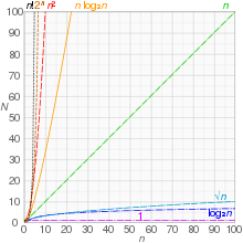
Running Time (film)analysis of algorithmstheoretical computer sciencecomputational complexityalgorithmconstant factorworst-case time complexityaverage-case complexityfunctionasymptotic behaviorbig O notationComputational complexity of mathematical operationsComplexity classinverse AckermannAmortized timedisjoint setiterated logarithmicDistributed coloring of cyclespriority queueDLOGTIMEBinary searchRange searchingk-d treeKadane's algorithmLinear searchSeidelpolygon triangulationcomparison sortFast Fourier transformBubble sortInsertion sortDirect convolutionpartial correlationKarmarkar's algorithmlinear programmingAKS primality testapproximation algorithmSteiner tree problemparity gamegraph isomorphismBest classical algorithminteger factorizationtraveling salesman problemdynamic programmingbrute-force searchEXPTIMEmatrix chain multiplication2-EXPTIMEPresburger arithmeticoperationelementLogarithmic growthbinary treesdictionaryalphabetical orderfloor functionpolylogarithmicmatrix chain orderingparallel random-access machinea graphdetermined to be planarfully dynamicapproximatelyproperty testingstatisticsParallel algorithmsguaranteed assumptionsdata structuresparallelismcontent-addressable memoryBoyer–Moore string-search algorithmUkkonen's algorithmsoft O notationIn-place merge sortQuicksortHeapsortmerge sortintrosortsmoothsortpatience sortingFast Fourier transformsMonge arraybinary tree sortbinary treeself-balancing binary search treeComparison sortsStirling's approximationrecurrence relationsorting algorithmsshell sortP (complexity)upper boundedpolynomialProblemscomputational complexity theoryCobham's thesisselection sortMaximum matchingsgraphsoptimizationstrongly polynomial timedecision problemsdeterministic Turing machinenon-deterministic Turing machineprobabilistic Turing machinequantum Turing machinerobustabstract machineAdleman–Pomerance–Rumely primality testP versus NP problemNP-completeQuasi-polynomial timequasi-polynomial growthexponential timeplanted cliquefind a large cliquerandom graphcomputational hardness assumptiongame theorymachine learningP versus NPexponential time hypothesisapproximation algorithmsset coversub-exponentialgeneral number field sieve