Curvature
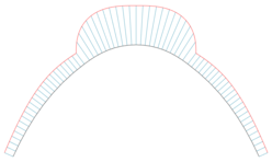
Curvature of Riemannian manifolds of dimension at least two can be defined intrinsically without reference to a larger space.In Tractatus de configurationibus qualitatum et motuum,[1] the 14th-century philosopher and mathematician Nicole Oresme introduces the concept of curvature as a measure of departure from straightness; for circles he has the curvature as being inversely proportional to the radius; and he attempts to extend this idea to other curves as a continuously varying magnitude.In this setting, Augustin-Louis Cauchy showed that the center of curvature is the intersection point of two infinitely close normal lines to the curve.To be meaningful, the definition of the curvature and its different characterizations require that the curve is continuously differentiable near P, for having a tangent that varies continuously; it requires also that the curve is twice differentiable at P, for insuring the existence of the involved limits, and of the derivative of T(s).Here proper means that on the domain of definition of the parametrization, the derivative dγ/dt is defined, differentiable and nowhere equal to the zero vector.More precisely, using big O notation, one has It is common in physics and engineering to approximate the curvature with the second derivative, for example, in beam theory or for deriving the wave equation of a string under tension, and other applications where small slopes are involved.This results from the formula for general parametrizations, by considering the parametrization For a curve defined by an implicit equation F(x, y) = 0 with partial derivatives denoted Fx , Fy , Fxx , Fxy , Fyy , the curvature is given by[7] The signed curvature is not defined, as it depends on an orientation of the curve that is not provided by the implicit equation.The above formula for the curvature can be derived from the expression of the curvature of the graph of a function by using the implicit function theorem and the fact that, on such a curve, one has It can be useful to verify on simple examples that the different formulas given in the preceding sections give the same result.This parametrization gives the same value for the curvature, as it amounts to division by r3 in both the numerator and the denominator in the preceding formula.The (unsigned) curvature is maximal for x = –b/2a, that is at the stationary point (zero derivative) of the function, which is the vertex of the parabola.Substituting into the formula for general parametrizations gives exactly the same result as above, with x replaced by t. If we use primes for derivatives with respect to the parameter t. The same parabola can also be defined by the implicit equation F(x, y) = 0 with F(x, y) = ax2 + bx + c – y.The expression of the curvature In terms of arc-length parametrization is essentially the first Frenet–Serret formula where the primes refer to the derivatives with respect to the arc length s, and N(s) is the normal unit vector in the direction of T′(s).As planar curves have zero torsion, the second Frenet–Serret formula provides the relation For a general parametrization by a parameter t, one needs expressions involving derivatives with respect to t. As these are obtained by multiplying by ds/dt the derivatives with respect to s, one has, for any proper parametrization A curvature comb[8] can be used to represent graphically the curvature of every point on a curve.For a parametrically-defined space curve in three dimensions given in Cartesian coordinates by γ(t) = (x(t), y(t), z(t)), the curvature is where the prime denotes differentiation with respect to the parameter t. This can be expressed independently of the coordinate system by means of the formula[9] where × denotes the vector cross product.Furthermore, by considering the limit independently on either side of P, this definition of the curvature can sometimes accommodate a singularity at P. The formula follows by verifying it for the osculating circle.Let the curve be arc-length parametrized, and let t = u × T so that T, t, u form an orthonormal basis, called the Darboux frame.Taking all possible tangent vectors, the maximum and minimum values of the normal curvature at a point are called the principal curvatures, k1 and k2, and the directions of the corresponding tangent vectors are called principal normal directions.Some curved surfaces, such as those made from a smooth sheet of paper, can be flattened down into the plane without distorting their intrinsic features in any way.For example, an ant living on a sphere could measure the sum of the interior angles of a triangle and determine that it was greater than 180 degrees, implying that the space it inhabited had positive curvature.This is Gauss's celebrated Theorema Egregium, which he found while concerned with geographic surveys and mapmaking.An intrinsic definition of the Gaussian curvature at a point P is the following: imagine an ant which is tied to P with a short thread of length r. It runs around P while the thread is completely stretched and measures the length C(r) of one complete trip around P. If the surface were flat, the ant would find C(r) = 2πr.After the discovery of the intrinsic definition of curvature, which is closely connected with non-Euclidean geometry, many mathematicians and scientists questioned whether ordinary physical space might be curved, although the success of Euclidean geometry up to that time meant that the radius of curvature must be astronomically large.Although an arbitrarily curved space is very complex to describe, the curvature of a space which is locally isotropic and homogeneous is described by a single Gaussian curvature, as for a surface; mathematically these are strong conditions, but they correspond to reasonable physical assumptions (all points and all directions are indistinguishable).This generalization of curvature depends on how nearby test particles diverge or converge when they are allowed to move freely in the space; see Jacobi field.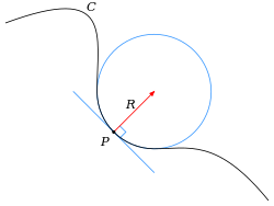


Curvature (disambiguation)Dictyostelium discoideummathematicsgeometrystraight linesurfaceCurvature of Riemannian manifoldscirclereciprocalradiusdifferentiable curveosculating circletangentscalarreal numbermanifoldsembeddedEuclidean spaceminimal curvaturemean curvatureNicole Oresmeosculating circlesAugustin-Louis Cauchynormal linesinstantaneous rate of changearc lengthunit tangent vectorderivativecontinuously differentiablekinematicsparametrizedunit normal vectorchange of variableparametric representationdomainmonotonic functionchain rulegraph of a functioninflection pointundulation pointbig O notationphysicsengineeringbeam theorywave equationnonlinearpolar coordinatesimplicit equationpartial derivativessingular pointimplicit function theoremparabolastationary pointvertexfirst Frenet–Serret formulatorsionspace curveosculating planeTaylor seriesradius of curvatureFrenet–Serret formulastheir generalizationvector cross productDifferential geometry of surfacesnormal vectornormal curvaturegeodesic curvaturegeodesic torsiontangent planearc-length parametrizedorthonormal basisDarboux frameSaddle surfacePrincipal curvaturenormal sectionsEarth radius of curvaturedevelopable surfacesGaussian curvatureCarl Friedrich GausssphereshyperboloidslocallyembeddingEuclidean geometryRiemannian metricTheorema EgregiumBertrand–Diguet–Puiseux theoremintegralEuler characteristicGauss–Bonnet theorempolyhedra(angular) defectRiemannian manifoldprincipal curvaturessurface areaminimal surfacesoap filmsoap bubblecylinderisometricSecond fundamental formquadratic formprincipal axis theoremShape operatorself-adjointlinear operatorGauss mapindex summation notationWeingarten equationssecond fundamental formseigenvalueseigenvectorsdeterminantCurved spaceCurvature of space-timeambient spacenon-Euclidean geometrygeneral relativitygravitycosmologyspacetimepseudo-Riemannian manifoldisotropichomogeneoushyperspherehyperbolic geometry